1. 理论
输入
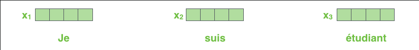
embedding words
turning each input word into a vector using an embedding algorithm.
问题:The size of this list is hyperparameter we can set – basically it would be the length of the longest sentence in our training dataset.
最底层的编码器输入是 embedding words,其后都是其他编码器的输出
In the bottom encoder that would be the word embeddings, but in other encoders, it would be the output of the encoder that’s directly below
BERT实践中也提到了这个,可以查看下
存疑
There are dependencies between these paths in the self-attention layer. The feed-forward layer does not have those dependencies, however, and thus the various paths can be executed in parallel while flowing through the feed-forward layer.
If you’re familiar with RNNs, think of how maintaining a hidden state allows an RNN to incorporate its representation of previous words/vectors it has processed with the current one it’s processing.
Self-Attention
作用:
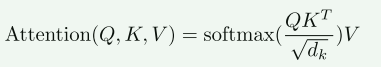
注意力机制:用于搞定当前处理的词与所有词的关系
Self-attention is the method the Transformer uses to bake the “understanding” of other relevant words into the one we’re currently processing.
As the model processes each word (each position in the input sequence), self attention allows it to look at other positions in the input sequence for clues that can help lead to a better encoding for this word.
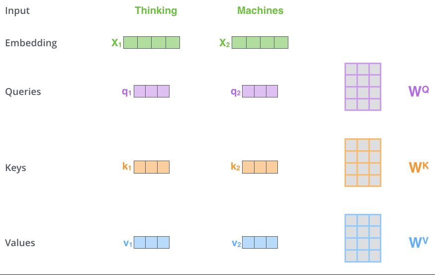
过程:
由Embedding产生QKV(长度不必同输入相同),当前词的Q与每个词(包含自身)的K做点积,再除以当前向量(指QKV)长度,取softmax(化为0-1的值),再将softmax的值(多个值1)同各自的V相乘,再累加,即可得到一个新的上下文向量V,该向量为包含当前词与所有词(包括自身)内容的向量,此时,该V中,与当前词相关度高的我们再把此V向量送入feed-forward neural network
They don’t HAVE to be smaller, this is an architecture choice to make the computation of multiheaded attention (mostly) constant.
计算方法:
一次矩阵运算得出所有X对应的新V
将所有输入词堆叠为一个矩阵,然后分别乘以一个权重得到 QKV
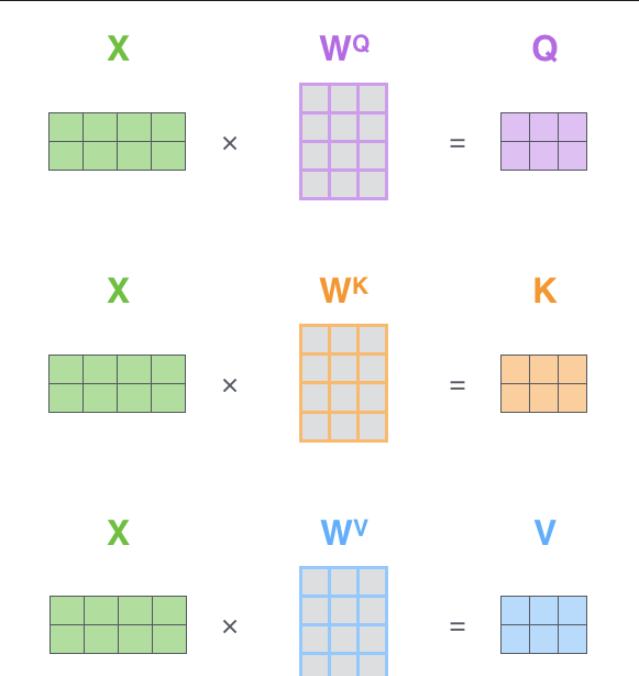
so,一次运算得出所有的V
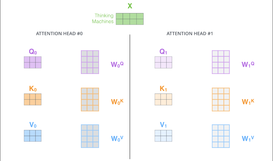
The Beast With Many Heads
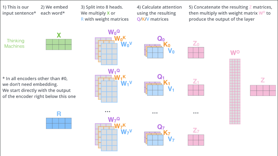
用多组不同的$W^Q, W^K, W^V$与X乘得到多组QKV,这些QKV并行运算的到多个V
It gives the attention layer multiple “representation subspaces”. with multi-headed attention we have not only one, but multiple sets of Query/Key/Value weight matrices
接下来通过按列拼接将这些V拼接为一个更宽的矩阵,在将此矩阵与一个新权重矩阵 $W^O$相乘得到最终的矩阵,该矩阵送入下一层,可以发现Z和X大小一致
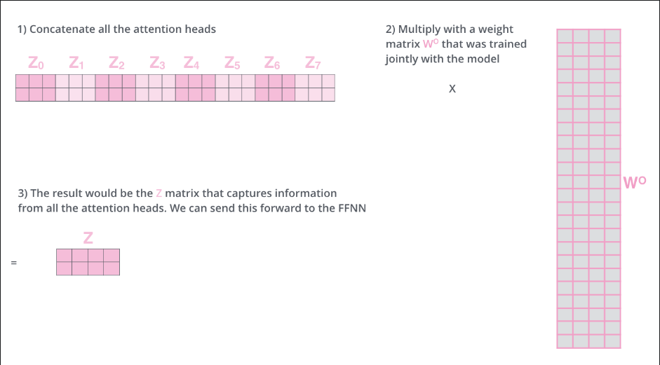
多头注意力机制矩阵计算全过程(多头是8个头哦)
注意力机制的输入与输出
举例输入维度为(2, 3, 512),这里是2句话,每句话3个词,d=512,即每个词的维度
| 步骤 | 操作 | 输入形状 | 输出形状 | 物理含义 |
|---|---|---|---|---|
| 0 | Input | - | (2, 3, 512) | 原始词向量 |
| 1 | Wq, Wk, Wv | (2, 3, 512) | (2, 3, 512) | 投影到特征空间 |
| 2 | Split Heads | (2, 3, 512) | (2, 8, 3, 64) | 拆分:8 个平行小脑 |
| 3 | Attention | (2, 8, 3, 64) | (2, 8, 3, 64) | 思考:在各自空间内聚合信息 |
| 4 | Merge Heads | (2, 8, 3, 64) | (2, 3, 512) | 拼接:物理合并结果 |
| 5 | Dense ($W^O$) | (2, 3, 512) | (2, 3, 512) | 融合:混合信息,恢复语义 |
举例shape=(2, 3, 512)的输入,这里是2句话,每句话3个词
# 这是一个 shape=(2, 3, 512) 的 Tensor 数据结构示意图

tensor_data = [
    # -------------- 第 1 句话 (Batch 0: "I love AI") --------------
    [
        # 第 1 个词 "I" 的 512 个特征
        [0.1, 0.2, -0.5, ..., 0.9],

        # 第 2 个词 "love" 的 512 个特征
        [0.8, 0.9, 0.1, ..., -0.1],

        # 第 3 个词 "AI" 的 512 个特征
        [-0.2, 0.5, 0.9, ..., 0.0]
    ],

    # -------------- 第 2 句话 (Batch 1: "He runs fast") --------------
    [
        # 第 1 个词 "He" 的 512 个特征
        [0.1, 0.1, -0.6, ..., 0.8],

        # 第 2 个词 "runs" 的 512 个特征
        [0.7, -0.2, 0.4, ..., 0.3],

        # 第 3 个词 "fast" 的 512 个特征
        [0.2, 0.3, 0.1, ..., -0.5]
    ]
]
划分多头后(2,8,3,64),对于一个词而言,每个头分别拿64个不同的维度
# Batch 0: "I love AI"
data_batch_0 = [
    # ---- 专家 0 (Head 0) 的视角 ----
    [
        # "I" 的特征 (前64个)
        [0.1, -0.2, ..., 0.5],
        # "love" 的特征 (前64个)
        [0.8, 0.9, ..., 0.1],
        # "AI" 的特征 (前64个)
        [-0.3, 0.4, ..., 0.0]
    ],

    # ---- 专家 1 (Head 1) 的视角 ----
    [
        # "I" 的特征 (第65-128个)
        [0.5, 0.1, ..., -0.2],
        # "love" 的特征 (第65-128个)
        [-0.1, 0.2, ..., 0.8],
        # "AI" 的特征 (第65-128个)
        [0.9, -0.5, ..., 0.3]
    ],

    # ... 中间省略 Head 2 到 Head 6 ...

    # ---- 专家 7 (Head 7) 的视角 ----
    [
        # "I" 的特征 (最后64个)
        [...],
        # "love" 的特征 (最后64个)
        [...],
        # "AI" 的特征 (最后64个)
        [...]
    ]
]
2 句话 $\times$ 8 个头 = 16 个独立空间,每个头看到的是该句子的一个方面,代码 tf.matmul(Q, K),在 GPU 内部是同时处理这 16 个独立的矩阵乘法
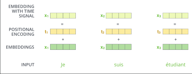
Positional Encoding
输入加入位置信息,让后序计算QKV时,能够感知该词的位置,如绝对位置: “这个词是在句首还是句尾?”相对距离: “词 A 和词 B 是紧挨着的,还是隔得很远?”
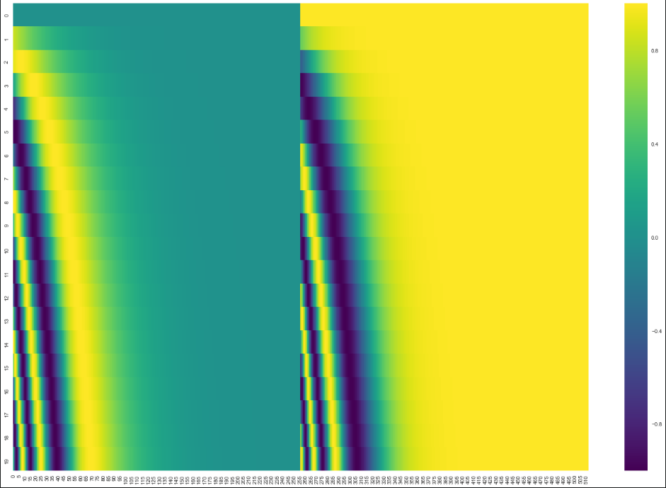
位置编码向量的生成
例如Tensor2Tensor 中的位置编码:
20个维度为512的位置编码,左边用sin计算,右边用cos计算,之后进行左右拼接得到整个编码
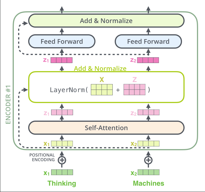
The Residuals
编码器中的体现
解码器中的体现
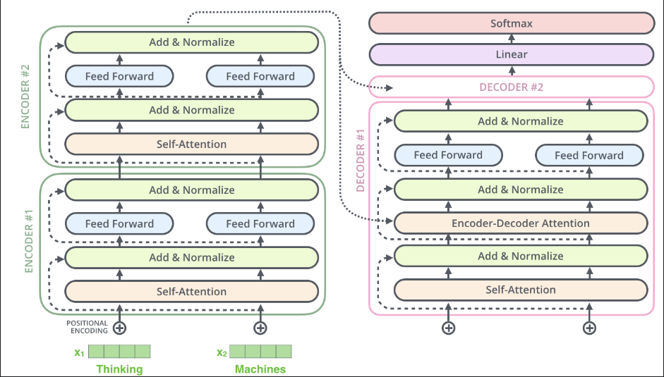
Decoder
最后一层编码器的输出变成一组K,V,传入“encoder-decoder attention” layer(解码器中间那层),具体来说Encoder 的输出会被“广播”(Broadcast)给6个中间的解码器层(因为叠加了6层解码器)。然而Q是来自Masked multi-attention layer,K,V包含了句子中提取的全部信息,一个相当于摘要,一个相当于具体的上下文,这样利用Masked multi-attention layer传来的Q,来从丰富的上下文中提取解码器感兴趣的信息,(这里是通过注意力机制完成的)
The output of the top encoder is then transformed into a set of attention vectors K and V. These are to be used by each decoder in its “encoder-decoder attention” layer which helps the decoder focus on appropriate places in the input sequence
Mask操作(这里对QdotK后的矩阵Z进行操作)
在 Softmax 之前,加上一个上三角矩阵(Mask Matrix)。这个矩阵规定:**凡是该位置之后的词,分数统统设为 $-\infty$(负无穷大)。
这样再经过softmaxt 上三角值就为0($e^{-\infty} \approx 0$)
 **
**
具体操作为:$\text{Softmax}(\text{Scores} + \text{Mask})$
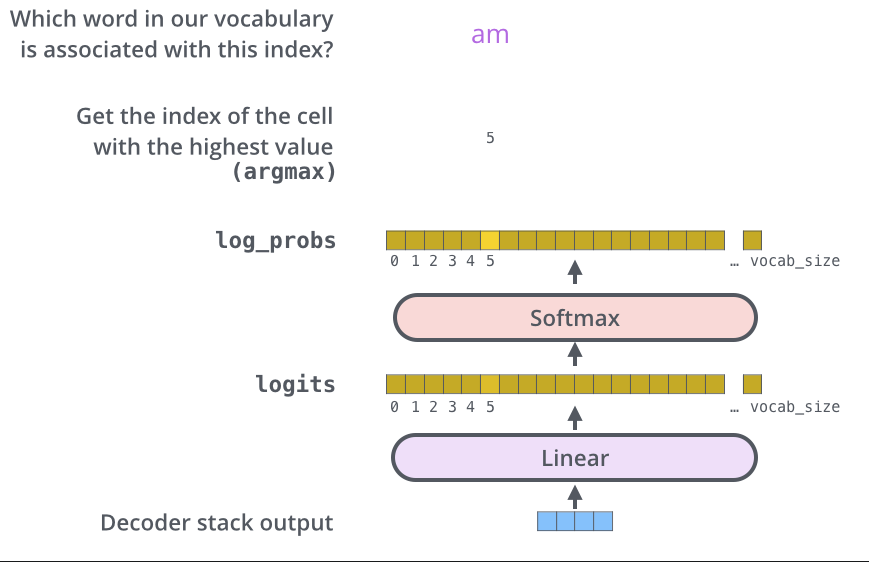
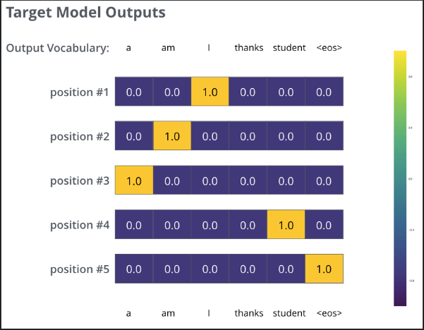
Final Linear and Softmax Layer
将floats向量转换为具体文字
The decoder stack outputs a vector of floats. How do we turn that into a word? That’s the job of the final Linear layer which is followed by a Softmax Layer.
The Linear layer is a simple fully connected neural network that projects the vector into a much, much larger vector called a logits vector.
全连接层进行投影,将输出投影到1*10000的向量(目的是为词汇表中每个词打个分)
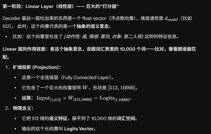
softmax层将打分转换为概率

我们从输出中调出概率最大的那个,便是预测词的index
one-hot编码&输出
词汇表
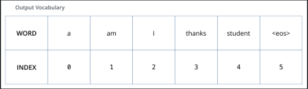
用one-hot后的index表示一个词
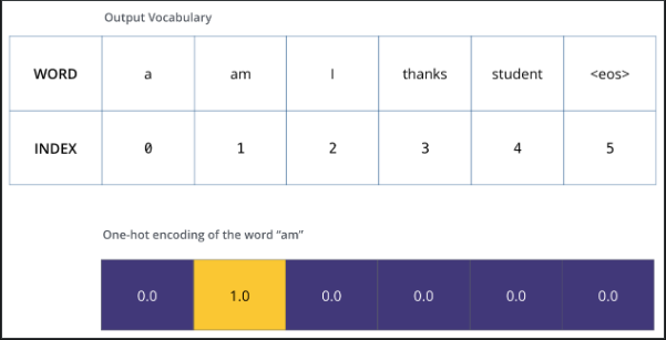
渴望的最终输出
代码部分
多头注意力机制
import numpy as np
import tensorflow as tf
from tensorflow.keras.layers import Layer
from tensorflow.keras.layers import Dense
from tensorflow.keras.layers import Softmax


class MultiAttention(Layer):
  def __init__(self, d_model, num_heads):
    super().__init__()
    self.d_model = d_model#d_model这里为512
    self.num_heads = num_heads#划分到8个头,每个头64

    #每个头的维度
    self.d_head = self.d_model // self.num_heads
    #初始化Wqkv矩阵
    #框架默认会给它们分配相互独立的、随机初始化的权重矩阵(W^Q, W^K, W^V)。 这些矩阵(以及它们的偏置 Bias)会在训练中得到更新
    self.Wq = Dense(self.d_model)
    self.Wk = Dense(self.d_model)
    self.Wv = Dense(self.d_model)
    #定义W^O
    self.dense = Dense(self.d_model)

  def attention(self,query,key,value,mask=None):

    # key_dim = tf.cast(tf.shape(key)[-1], tf.float32)
    key_dim = self.d_head #这里直接获取head的维度来替换上句
    #softmax内的部分
    scaled_scores = tf.matmul(query,key,transpose_b=True)/np.sqrt(key_dim)

    #若是mask attenntion
    # 则在softmax前进行替换,将不该看见的内容替换为负无穷
    if mask is not None:
      scaled_scores = tf.where(mask==0, -np.inf, scaled_scores) #将得分中mask为0的部分替换为负无穷
    weights = Softmax(scaled_scores)
    return tf.matmul(weights, value), weights #注意这里权重矩阵在生产环境中,不用返回

  def split_heads(self,x):
    batch_size = x.shape[0]
    x_split = tf.reshape(x,(batch_size,-1,self.num_heads,self.d_head))#将输入x改造为指定格式(批量大小,序列长度,头数,头维度),-1代表1自适应
    return tf.transpose(x_split, perm=[0,2,1,3])#对维度进行重排,将Head维度移动到Sequence Length维度之前

  #逆转上一个函数
  def merge_heads(self, x):
    x_merge = tf.transpose(x,perm=[0,2,1,3])
    return tf.reshape(x_merge,(batch_size,-1,self.d_model))#改变为输入时的(批量大小,序列长度,输入维度),其中批量大小对应X的行数,序列长度对应句子中词的数量,输入维度是每个词用多大的维度来表示(这里是512)

  #but why?
  def call(self,q,k,v,mask):
    # 初始化QKV
    Q = self.Wq(q)
    V = self.Wv(v)
    K = self.Wk(k)
    #那么划分多头究竟是在干什么:
    #原来的 512 维是一个大杂烩。
    #现在拆成 8 个 64 维的小组
    Q = self.split_heads(Q)
    K = self.split_heads(K)
    V = self.split_heads(V)
    output, weights = self.attention(Q,K,V,mask)#8个头互不干扰,各自在自己的 64 维空间里算出谁和谁关系好(Score),并提取出相应的信息(Value)。
    #这是合并为大Z
    output = self.merge_heads(output)#Concat,简单的拼接z,得到Z
    return self.dense(output),weights#$W^O$ 就对应 self.dense, Z*W^O得到最终的多头注意力机制输出
编码器块
class EncoderBlock(Layer):
  def __init__(self, d_model, num_heads, hidden_dim, dropout_rate=0.1):
    super().__init__()
    self.mhaa = MultiAttention(d_model,num_heads)
    self.ffn = self.feed_forward_neural_network(d_model,hidden_dim)


    self.dropout1 = tf.keras.layers.Dropout(dropout_rate)#在每一次训练的迭代中,随机让 10% 的神经元暂时“闭嘴”(输出置为 0),不参与这一次的工作。
    self.dropout2 = tf.keras.layers.Dropout(dropout_rate)

    self.layernorm1 = tf.keras.layers.LayerNormalization()
    self.layernorm2 = tf.keras.layers.LayerNormalization()
  def feed_forward_neural_network(self,d_model, hidden_dim):
    return tf.keras.Sequential(

      [tf.keras.layers.Dense(hidden_dim, activation='relu'),#维度变化: d_model (512) to hidden_dim (2048)
      #ReLU 会把所有负数值变成 0。这相当于在宽阔的高维空间里,对特征进行了一次筛选和提纯,只保留有用的激活模式
      tf.keras.layers.Dense(d_model)#维度变化: hidden_dim (2048) to d_model (512)。
       #动作: 把刚才在高维空间处理好的特征,重新压缩回原来的 512 维。为了让数据能塞回“主干道”(Residual Connection),传给下一层
       ]
    )

  def call(self, x, mask):
    mha_output, attention_weights = self.mha(x,x,x,mask)
    #因为 MultiHeadAttention 这个组件太通用了,它必须显式地接收 Query、Key、Value 三个输入
    #而在 EncoderBlock 中,我们使用的是 “自注意力”,所以这三个输入恰好都是同一个 x
    mah_output = self.dropout1(mha_output)
    mah_output = self.layernorm1(x+mha_output)#残差连接Add ,层归一化Norm

    #前馈神经网络
    ffn_output = self.ffn(mha_output)
    ffn_output = self.dropout2(ffn_output)
    output = self.layernorm2(mha_output + ffn_output)
    return output, attention_weights
编码器
class Encoder(Layer):

  def __init__(self, num_blocks, d_model, num_heads, hidden_dim, src_vocab_size, max_seq_len, dropout_rate=0.1):
    super().__init__()
    self.d_model = d_model
    self.max_seq_len = max_seq_len

    self.token_embed = tf.keras.layers.Embedding(src_vocab_size, self.d_model)
    self.positional_embed = tf.keras.layers.Embedding(max_seq_len,self.d_model)#现代的可学习编码,而不是原文正余弦位置编码

    self.dropout = tf.keras.layers.Dropout(dropout_rate)
    self.blocks = [EncoderBlock(self.d_model,num_heads,hidden_dim,dropout_rate) for _ in range(num_blocks)]#循环创建编码器块


  def call(self, input, mask):
    token_embeds = self.token_embed(input)

    num_pos = input.shape[0] * self.max_seq_len #算出整个 Batch 一共有多少个单词位置需要填。
    pos_idx = np.resize(np.arange(self.max_seq_len), num_pos)#生成并平铺索引eg:[0,1,2]根据num_pos/max_seq_len的值进行重复,如[0,1,2,0,1,2...]
    pos_idx = np.reshape(pos_idx, input.shape)#重塑形状为:[[0, 1, 2],[0, 1, 2]]
    pos_embeds = self.pos_embed(pos_idx)

    x = self.dropout(token_embeds+pos_embeds

                     )
    for block in self.blocks:
      x, weights = block(x,mask)

    return x,weights
解码器块
class DecoderBlock(Layer):
  def __init__(self, d_model, num_heads, hidden_dim, dropout_rate=0.1):
    super().__init__()
    #两个多头
    self.mha1 = MultiAttention(d_model,num_heads)
    self.mha2 = MultiAttention(d_model,num_heads)

    self.ffn = self.feed_forward_neural_network(d_model,hidden_dim)
    #让一定比例的参数不参与学习,目的是防止过拟合
    self.dropout1 = tf.keras.layers.Dropout(dropout_rate)
    self.dropout2 = tf.keras.layers.Dropout(dropout_rate)
    self.dropout3 = tf.keras.layers.Dropout(dropout_rate)
    #用Add&Norm
    self.layernorm1 = tf.keras.layers.LayerNormalization()
    self.layernorm2 = tf.keras.layers.LayerNormalization()
    self.layernorm3 = tf.keras.layers.LayerNormalization()
  #ffn
  def feed_forward_neural_network(self, d_model, hidden_dim):
    return tf.keras.Sequential([tf.keras.layers.Dense(hidden_dim,activation='relu'),
                                tf.keras.layers.Dense(d_model)])
  def call(self, encoder_output, target, decoder_mask, memory_mask):
    mha_output1,attention_weights = self.mha1(target,target,target,decoder_mask)#这里target是?
    mha_output1 = self.dropout1(mha_output1)
    #Add&Norm
    mha_output1 = self.layernorm1(mha_output1 + target)
    #将编码器的输出传入,多头中会自动计算出K,V,而Q是由上一层的Masked Multi-Head Attention提供
    mha_output2,attention_weights = self.mha2(mha_output1, encoder_output,encoder_output,memory_mask)

    mha_output2 = self.dropout2(mha_output2)
    #Add&Norm
    mha_output2 = self.layernorm2(mha_outpt2 + mha_output1)

    ffn_output = self.ffn(mha_output2)
    ffn_output = self.dropout3(ffn_output)

    #Add&Norm
    output = self.layernorm3(ffn_output + mha_output2)
    return output, attention_weights
解码器
class Decoder(Layer):
  def __init__(self, num_blocks, d_model, num_heads, hidden_dim, target_vocab_size, max_seq_len, dropout_rate=0.1):
    super().__init__()
    self.d_model = d_model
    self.max_seq_len = max_seq_len
    #了解这两个embedding
    self.token_embed = tf.keras.layers.Embedding(target_vocab_size, self.d_model)
    self.pos_embed = tf.keras.layers.Embedding(max_seq_len, self.d_model)
    self.dropout = tf.keras.layers.Dropout(dropout_rate)
    self.blocks = [DecoderBlock(d_model, num_heads, hidden_dim, dropout_rate) for _ in range(num_blocks)]

  def call(self, encoder_output, target, decoder_mask, memory_mask):
    token_embeds = self.token_embed(target)
    #标明每个词在句子中的位置
    num_pos = target.shape[0] * self.max_seq_len
    pos_idx = np.resize(np.arange(self.max_seq_len),num_pos)
    pos_idx = np.reshape(pos_idx, target.shape)
    pos_embeds = self.pos_embed(pos_idx)

    x = self.dropout(token_embeds+pos_embeds)

    for block in self.blocks:
      #这里是对每个解码器都传入了编码器的最后输出
      x,weights = block(encoder_output,x,decoder_mask, memory_mask)#memory_mask是什么
    return x,weights
构建transformer
import tensorflow as tf
from tensorflow.keras import Model

class Transformer(Model):
    def __init__(self, num_blocks, d_model, num_heads, hidden_dim, source_vocab_size,
                 target_vocab_size, max_input_len, max_target_len, dropout_rate=0.1):
        super().__init__()

        # 1. 编码器 (负责源语言/英文)
        # 用 source_vocab_size 和 max_input_len
        self.encoder = Encoder(num_blocks, d_model, num_heads, hidden_dim,
                               source_vocab_size, max_input_len, dropout_rate)

        # 2. 解码器 (负责目标语言/中文)
        # 必须传入 target_vocab_size 和 max_target_len
        self.decoder = Decoder(num_blocks, d_model, num_heads, hidden_dim,
                               target_vocab_size, max_target_len, dropout_rate)

        # 3. 输出层 (分类器) [修复缩进和拼写]
        # 它的神经元数量必须等于目标词表大小,这样才能预测下一个也是哪个词
        self.output_layer = tf.keras.layers.Dense(target_vocab_size)

    def call(self, input_seqs, target_input_seqs, encoder_mask, decoder_mask, memory_mask):
        # 1. 编码
        encoder_output, encoder_attention_weights = self.encoder(input_seqs, encoder_mask)

        # 2. 解码
        # [修复变量名]: target_inputs_seqs -> target_input_seqs
        # 注意:这里传入的是 encoder_output,供解码器做 Cross-Attention 用
        decoder_output, decoder_attention_weights = self.decoder(encoder_output,
                                                                 target_input_seqs,
                                                                 decoder_mask,
                                                                 memory_mask)

        # 3. 最终分类 (把 d_model 维度的向量映射回 词表维度)
        # decoder_output shape: (batch, seq_len, d_model)
        # final_output shape:   (batch, seq_len, target_vocab_size)
        final_output = self.output_layer(decoder_output)

        return final_output, encoder_attention_weights, decoder_attention_weights
LayerNorm 的作用就是强制把每个样本的特征数据“拉回”到一个标准的分布上:
均值为 0 (Centering)
方差为 1 (Scaling)
具体操作(在 512 维上操作)
对于 Transformer 中的每一个词向量(512维):
算出这 512 个数的平均值 ($\mu$)。
算出这 512 个数的标准差 ($\sigma$)。
标准化: 把这 512 个数都减去平均值,再除以标准差。
再缩放(关键一步): 乘上一个可学习参数 $\gamma$ (Scale),再加上一个可学习参数 $\beta$ (Shift)。
注意: 最后这一步“再缩放”是为了让模型自己决定是否需要保留一点原始的分布特征,而不是强制死板地全是 0 和 1。LayerNorm 的作用就是强制把每个样本的特征数据“拉回”到一个标准的分布上:
均值为 0 (Centering)
方差为 1 (Scaling)
具体操作(在 512 维上操作)
对于 Transformer 中的每一个词向量(512维):
算出这 512 个数的平均值 ($\mu$)。
算出这 512 个数的标准差 ($\sigma$)。
标准化: 把这 512 个数都减去平均值,再除以标准差。
再缩放(关键一步): 乘上一个可学习参数 $\gamma$ (Scale),再加上一个可学习参数 $\beta$ (Shift)。
注意: 最后这一步“再缩放”是为了让模型自己决定是否需要保留一点原始的分布特征,而不是强制死板地全是 0 和 1。
Feed Forward
为什么要这么折腾?(升维再降维)
可以把这个过程想象成 “拆解分析 -> 重新打包”:
Input (512): 比如单词向量包含了“苹果”这个概念。
Dense 1 (2048): 显微镜模式。把“苹果”这个概念拆解成 2048 个细微的属性:
是红色的吗?是。
是水果吗?是。
是科技公司吗?不是。
能吃吗?能。
… (铺开来看,寻找更细腻的特征组合)
ReLU: 过滤。把“是科技公司吗?不是”这种无关或负面的噪音去掉。
Dense 2 (512): 总结模式。根据刚才分析的细微属性,重新总结出一个更精炼的“苹果”向量,放回 512 维。
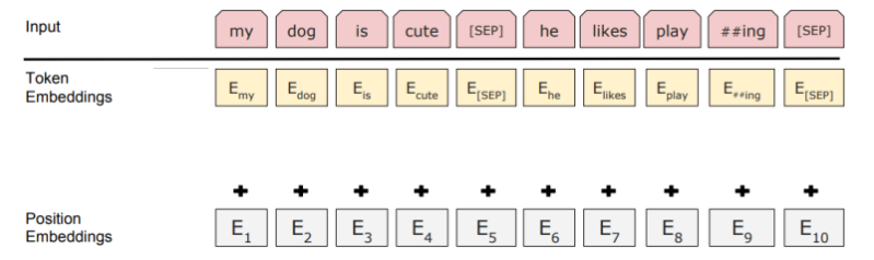
Position IDs 是句子中该词的位置
| 单词 (Token) | 我 | 喜欢 | 学 | 代码 |
|---|---|---|---|---|
| Token ID (查字表用) | 501 | 29 | 888 | 1024 |
| Position ID (查位置表用) | 0 | 1 | 2 | 3 |
处理后的输入大概是这个样子(图在BERT的基础上进行修改)
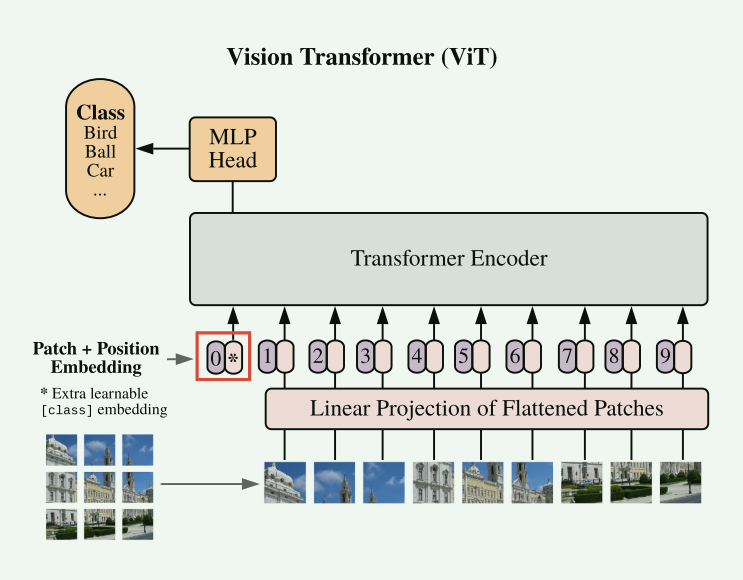
2.Vit
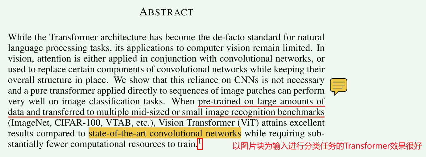
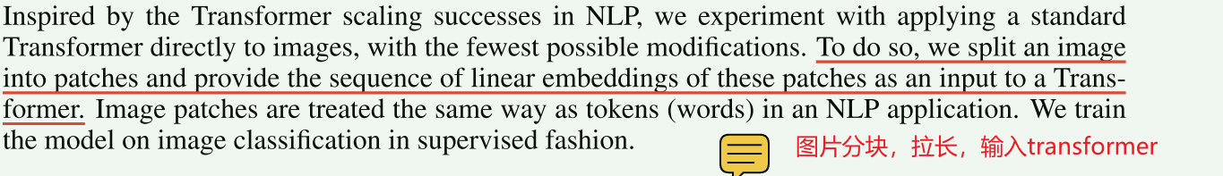
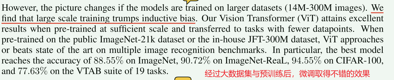
输入处理:图片切分为固定大小(16*16),展平,投影到transformer的输入维度D(512),附加位置Embedding和class embedding,后者用于分类任务
举个例子:
原始数据: 假设一个 $2 \times 2$ 的 RGB 图像块的像素值如下(为了简化,我们只用 3 个通道 $R, G, B$ 的值): $\begin{array}{ccc} \text{位置 (1,1)} & \text{位置 (1,2)} \\ R=10, G=20, B=30 & R=40, G=50, B=60 \\ \text{位置 (2,1)} & \text{位置 (2,2)} \\ R=70, G=80, B=90 & R=100, G=110, B=120 \end{array}$
展平向量 $x_i$: 将所有像素值按顺序排列成一个向量。
输入维度 $P^2 \cdot C = (2 \times 2) \times 3 = 12$
$x_i = [10, 20, 30, \ 40, 50, 60, \ 70, 80, 90, \ 100, 110, 120]^T \in \mathbb{R}^{12}$
模型定义了一个可学习的投影矩阵 $\mathbf{E}$,它将 12 维的输入映射到 8 维的特征空间 $D=8$。
- 投影矩阵 $\mathbf{E}$: $\mathbf{E} \in \mathbb{R}^{12 \times 8}$ (这个矩阵的 96 个值会在训练中被学习。)
通过矩阵乘法,我们计算图像块 $i$ 的嵌入向量 $z_i$。
计算公式: $z_i = x_i \mathbf{E}$
维度变化: $\underset{(1 \times 12)}{x_i} \ \ \ \underset{(12 \times 8)}{\mathbf{E}} \ \ \ \longrightarrow \ \ \ \underset{(1 \times 8)}{z_i}$
结果 $z_i$: $z_i$ 是一个 8 维的向量,例如: $z_i = [0.1, -0.5, 1.2, 0.8, -0.2, 1.5, -0.3, 0.4]^T \in \mathbb{R}^{8}$
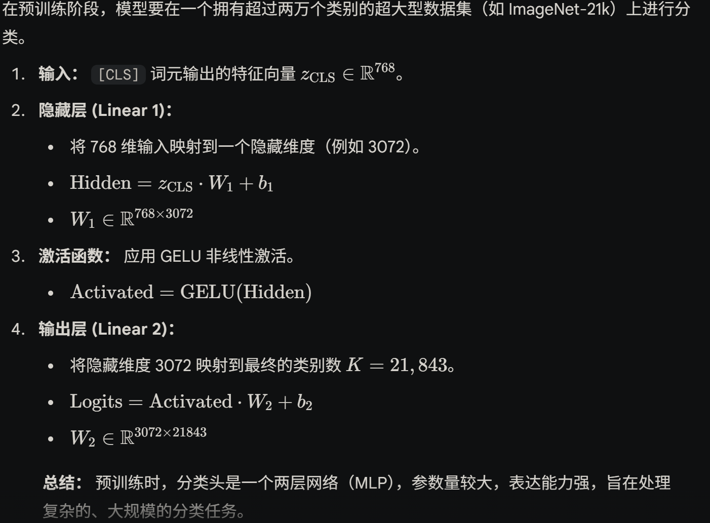
预训练时MLP有两层,经隐藏层映射到一个维度,再经过最后一层映射到分类维度(维度和分类数一致)
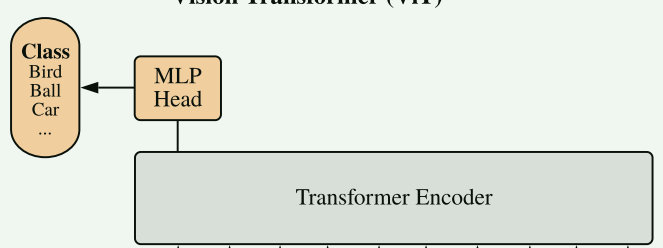
微调时的MLP Head 具体问题具体分析,移除预训练时使用的那个多层感知机(MLP)分类头,替换: 换上一个新的、单层的线性层(也称为前馈层,Feedforward Layer)。这个新层的权重矩阵维度是 $D \times K$,其中 $D$ 是 Transformer 编码器的特征维度(Hidden Size),$K$ 是下游任务的类别数量
不太理解这里对新的MLP Head 进行0初始化or随机初始化
BERT:Pre-training of Deep Bidirectional Transformers
BERT 是双向 Transformer”时,其实是在强调它保留了 Transformer Encoder 的原生特性,区别于 GPT 那种加了 Mask 的 Transformer Decoder。