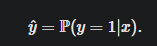
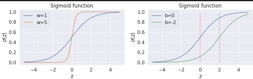
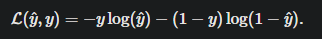
输入x希望输出y=1的可能性最大
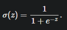
通过sigmod输出映射到0,1,其中0.5为分界线
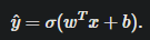
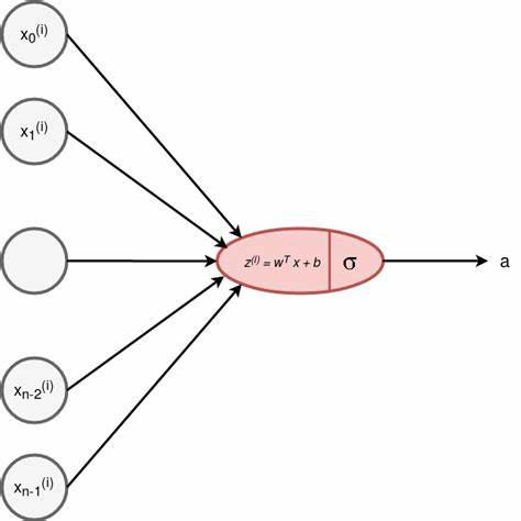
逻辑回归,使用sigmod为激活函数的神经网络
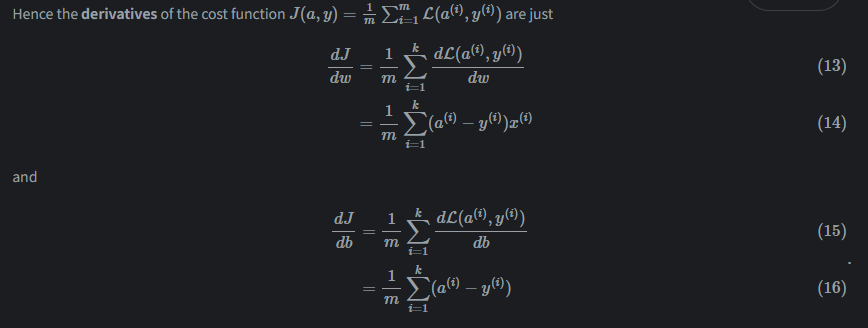
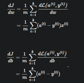
Evaluating the cost function can be thought of as forward propagation and computing derivatives can be thought of as backpropagation.
sigmod中权重越高,越自信,就是轻微的输入变化带来截然不同的结果
偏差的不同呢是的决策边界发生变化,就是说分界点改变了。
least squares不再适用(回归函数经过sigmoid,不再是Convex functions,即凸函数)
Convex functions have the useful property that any local minimum is also a global minimum
第一幅为Convex functions,第二幅为非 Convex functions,后者的局部最小值不一定是全局最小值
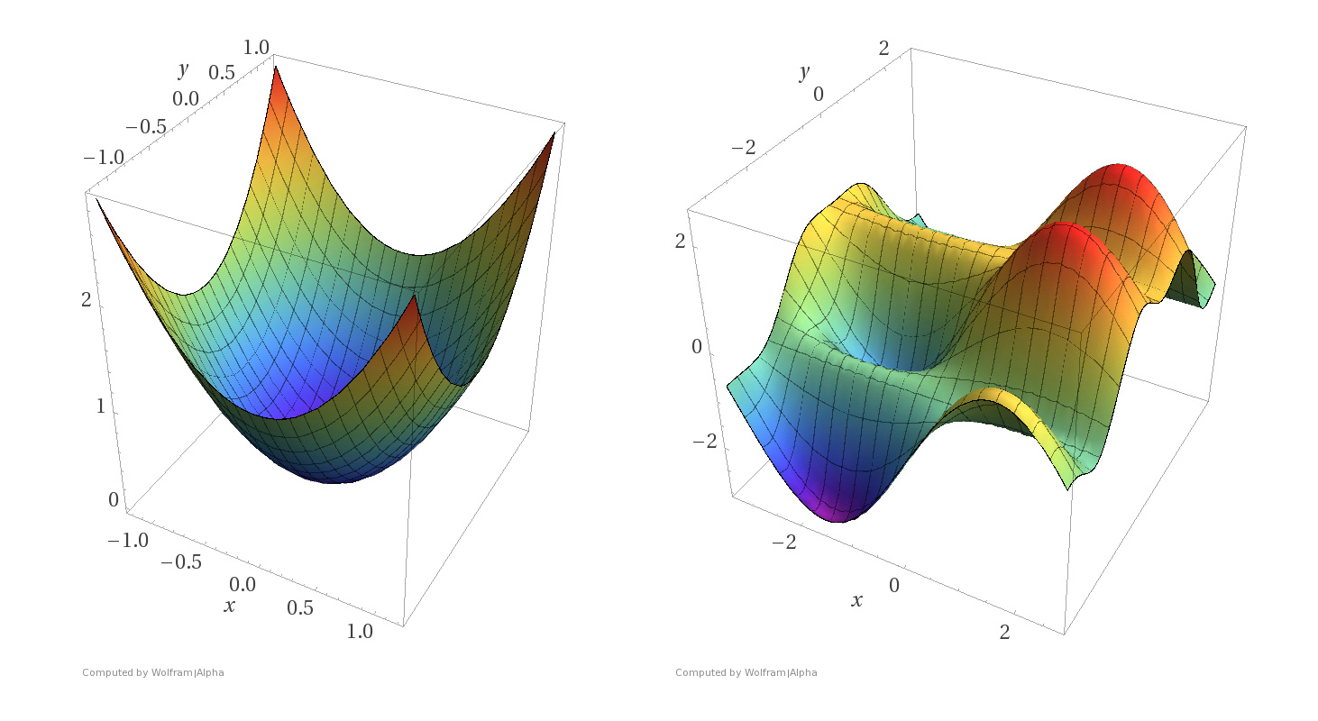
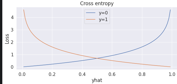
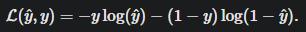
logistic regression 使用 cross-entropy loss,这是它的凸函数
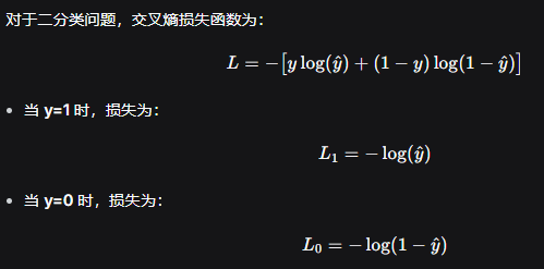
横轴预测值,竖轴损失:预测错误损失趋向无穷,预测正确损失为0
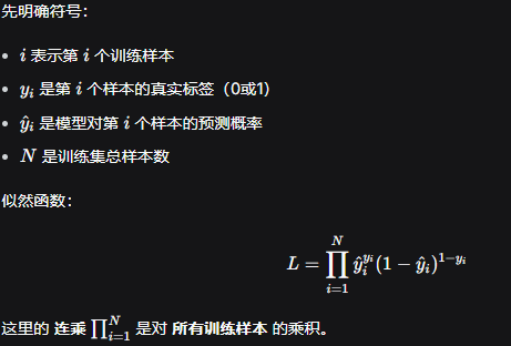
由最大似然 推出 交叉熵损失,
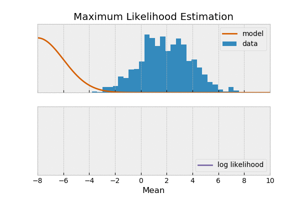
最大似然,思想是通过选择模型参数,使得 观测到的数据出现的概率最大。
为何可以写成?
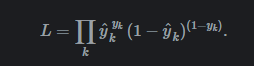
连乘内是伯努利分布的简化写法,如下:
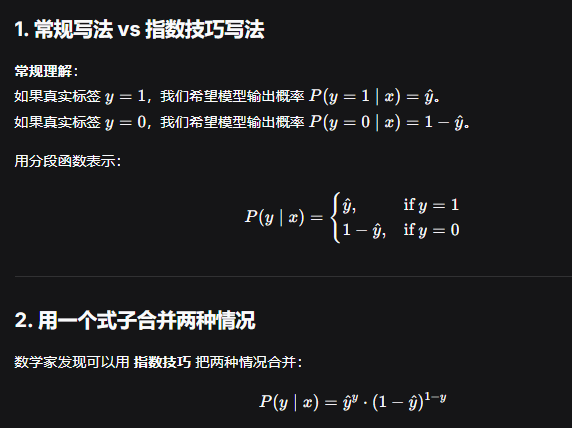
连乘是因为,对于每个样本,视为独立同分布,又独立事件的联合概率 = 各自概率的乘积,故此用连乘。
再次简化,log易于求导,且单调增(使得logL最大,必然使得L最大)
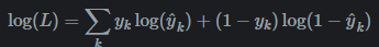
ai: 注意到,这里推出的logL是负数,取-logL即为交叉熵
梯度下降
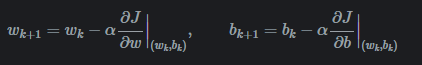
其中 α需要适中

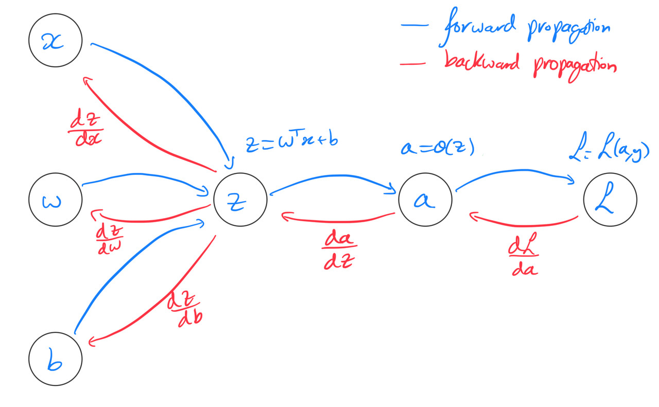
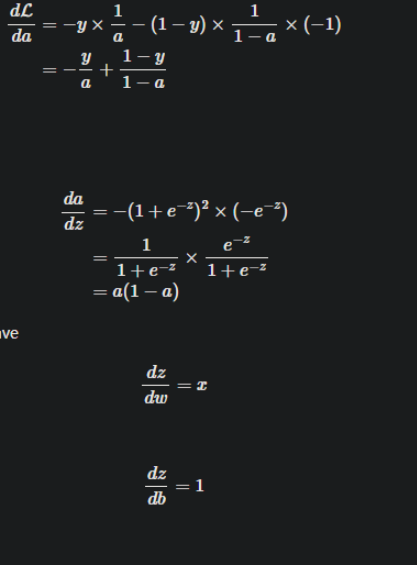
下面将用链式求导法则和计算图进行讲解:
通过一番推导(推导待补充)
我们得到:通计算图中的反向传播,得到db,dw.
逻辑回归的伪代码
Inputs: X, Y, alpha, K
Initialise w=np.zeros(len(X)), b=0
    For k=1, ..., K:
        Initialise: J=0, dw=0, db=0
        For i=1,...m:
            z=w.T@X[:,i]+b
            a=sigmoid(z)

            # Cost function
            J+=cross_entropy(a,Y[i])

            # Derivatives
            #这里要结合着计算图来看反向传播,
            dz=a-Y[i] #dz为 ∂l/∂z
            #X[:,i]为∂z/∂w,dz为 ∂l/∂z ,就是链式求导,求dl/dw
            dw+=X[:,i]*dz
            db+=dz #这里是因为 ∂z/∂b = 1,

        # Take average
        J/=m
        dw/=m
        db/=m

       # Gradient descent step
       w=w-alpha*dw
       b=b-alpha*db
       print(J)

   return w, b
可以借助下面的四幅图来看懂它
首先计算图
其次链式求导
再者交叉熵损失函数
矩阵形式表达的逻辑回归伪代码,不作多余解释,有疑问看上一个即可
Inputs: X, Y, alpha, K
Initialise w=np.zeros(len(X)), b=0
    For k=1, ..., K:
        Z=w.T@X+b
        A=sigmoid(Z)

        # Cost function
        J=-(np.dot(Y,np.log(A))+np.dot(1-Y,np.log(1-A)))/m

        # Derivatives
        dZ=A-Y
        dw=(X@dZ.T)/m
## 注意dz
        db=dZ.sum()/m

        # Gradient descent step
        w=w-alpha*dw
        b=b-alpha*db

        print(J)

    return w, b
实现逻辑回归by numpy
class logic_regression:
    #init
    #参数 学习率 k w b costs, verbose (训练过程可视化)
    def __init__(self, verbose=False, alpha=0.1, K= 100):
        self.verbose = verbose
        self.alpha = alpha
        self.K = K
        self.b = 0
        self.costs = []
        self.w = np.array([]) #创建空数组

    #fit
    def fit(self,X,y):
        m = len(y) #样本总数,下面求平均会损失会用到
        self.w = np.zeros(X.shape[1]) #X.shap[1]为特征的数量 旨在为每个特征初始化w
        for k in range(self.K):
            #1.前向传播
            # Z = self.w @ X.T + self.b
            Z = X @ self.w + self.b  # 修正:更标准的写法,避免转置
            A = 1/(1+np.exp(-Z)) #sigmod激活函数
            #2.损失计算
            cost = -(np.dot(y,np.log(A)) + np.dot((1-y),np.log(1-A))) / m #这里就是最大似然估计推出的  前方再方上一个负号 /m是取平均损失
            #3。梯度下降,反向传播
            dZ = A-y #反向传播 计算图 dl/dz
            dw = (X.T @ dZ) / m #
            db = np.sum(dZ) / m
            #4.更新参数
            self.w = self.w - self.alpha * dw
            self.b = self.b - self.alpha * db
            #5.统计损失
            self.costs.append(cost)
            # Print the cost every 100 iterations
            if (self.verbose) and (((k+1) % 100) == 0):
                print(f"Iteration = {k+1}, cost = {cost}")
    #predict
    #@return 0 1
    def predict(self,X_test):
        Z = X_test @ self.w + self.b
        A = 1/(1+np.exp(-Z))
        return np.around(A).astype(int)

    #predict_probability
    #@return 0-1
    def predict_probability(self,X_test):
        # Z = self.w @ X_test.T + self.b
        Z = X_test @ self.w + self.b  # 修正:更标准的写法
        A = 1/(1+np.exp(-Z))
        return A

    #score
    def score(self, X_test, y_test):
        res = self.predict(X_test)
        acc = (res == y_test).sum() / len(y_test)
        return acc
逻辑回归 by pytorch
Class封装model, 继承 nn.Module 并定义forward属性,以便调用pytorch的神经网络相关方法
When working with neural networks, we need to inherit the ‘nn.Module’ and define a ‘forward’ attribute.
The inheritance part is done to get access to attributes like ‘model.parameters()’, which are used in training.
class logistic_regression(nn.Module):
    #init
    def __init__(self,n_feats):#n_feats: 输入特征数量
        super().__init__() #调用父类进行初始化
        self.lin = nn.Linear(n_feats,1) #nn将自动创建权重 w 和偏置 b 这里1是输出维度
        self.sig = nn.Sigmoid()
    def forward(self,x):
        return self.sig(self.lin(x))
是不是少了什么? 损失?反向传播?
PyTorch 的设计哲学:模型、损失、优化器分离
Some of the basic PyTorch components include:
Tensors - N-dimensional arrays that serve as PyTorch’s fundamental data structure. They support automatic differentiation, hardware acceleration, and provide a comprehensive API for mathematical operations.
Autograd - PyTorch’s automatic differentiation engine that tracks operations performed on tensors and builds a computational graph dynamically to be able to compute gradients.
Neural Network API - A modular framework for building neural networks with pre-defined layers, activation functions, and loss functions. The
nn.Modulebase class provides a clean interface for creating custom network architectures with parameter management.DataLoaders - Tools for efficient data handling that provide features like batching, shuffling, and parallel data loading. They abstract away the complexities of data preprocessing and iteration, allowing for optimized training loops.
PyTorch 的设计理念:
🧩 模型 (nn.Module):只关心"如何预测"
📊 损失函数:只关心"预测得好不好"
⚙️ 优化器:只关心"如何改进参数"
🔄 训练循环:把它们组合起来工作
一下是pytorch的逻辑回归的完整实现
这里我们就可以知道为何model一定要继承nn.Module,为了调方法,为何必须实现forward前向传播,将数据传入module时将自动调用forwawrd
#0 定义模型
class logistic_regression(nn.Module):
    #init
    def __init__(self,n_feats):#n_feats: 输入特征数量
        super().__init__() #调用父类进行初始化
        self.lin = nn.Linear(n_feats,1) #nn将自动创建权重 w 和偏置 b 这里1是输出维度
        self.sig = nn.Sigmoid()
    def forward(self,x):
        return self.sig(self.lin(x))


#1. 交叉熵损失
loss = nn.BCELoss()

#2. 反向传播/梯度下降 自适应调整每个参数的学习率
optimiser = torch.optim.Adam(params = model.parameters(), lr=0.01) #params = model.parameters()  # 获取模型中所有的 w 和 b    lr=0.01学习率

#3.训练过程
n_iters = 2000 #训练回合

for epoch in range(n_iters):
    # Zero gradients 梯度清0,应在每轮训练回合开始时清0
    optimiser.zero_grad() #numpy实现时使用的是局部变量,故每回合开始自动梯度清0

    #1. Forward pass
    y_preds = model(X_train) #调用 model(X_train) 时,PyTorch 会自动调用模型的 forward 方法
    #2. 计算损失
    L = loss(y_preds, y_train)
    #3. Backprop
    L.backward() #实际是利用计算图进行反向传播

    #4. Update parameters
    optimiser.step() #更新参数 权重偏差等

    #5. Print loss
    if epoch % 20 == 0:
        print(f'Epoch {epoch}, loss {L.item():.3f}')