主要介绍LeNet 与 AlexNet,还 涉及到dropout, maxpooling, relu等概念
In this notebook we will motivate and implement from scratch two Convolutional Neural Networks (CNNs) that had big impacts on the field of Deep Learning. Namely, we will look at LeNet-5 (Yann LeCunn et al., 1989), which is considered one of the first CNNs ever and also AlexNet (Alex Krizhevsky et al., 2012), which won the 2012 ImageNet competition by an impressive marging and introduced many techniques that are considered state of the art even today (e.g. dropout, maxpooling, relu, etc).
These networks offer a glimpse into the history of computer vision, including the early trends and challenges. Limited computational resources in particular have led to the rapid innovation we’ve seen in the last few decades.

介绍概念
Convolutional layer
通过卷积核提取特征

Pooling layer
让特征图大小缩小(历史遗留问题,这里也称为下采样,有用池化层进行下采样,而现在用卷积层下采样),深层的视野“变大”
max pooling具有平移不变性,而 average pooling 仅可缩小特征图大小
故AlexNet中 Maxpooling is being used instead of average pooling.
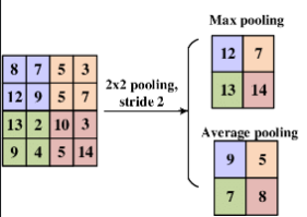
对于池化让感受视野变大的理解
Activation layer
非线性激活函数,enable the model to learn more complex relationships
AlexNet中使用ReLU which makes training much faster.
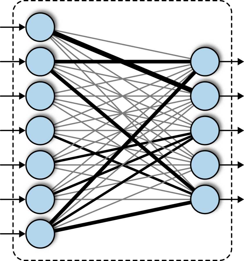
Dense layer ( fully connected layer)
every neuron in the previous layer is connected to the current layer through weights and biases.
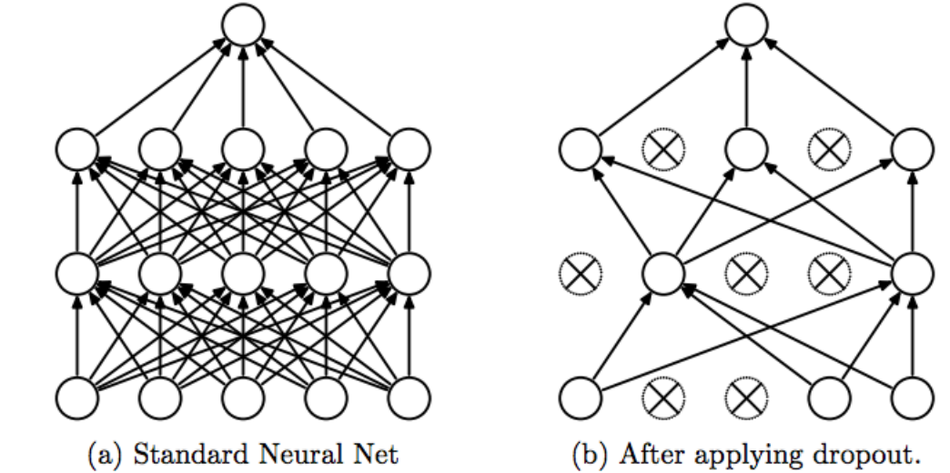
Dropout
随机断开几个神经网络连接,使得结果不仅仅依赖于哪几个神经元(也就是防止过拟合)
由AlexNet引入
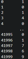
one-hot编码
原始字符标签,第一列是序号,第二列是标签
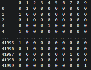
one-hot
第一列是序号,0-9中显示为1的是标签,eg:第0行1处显示1,则说明该行标签为1;第0、41999行9处显示1,则说明该行标签为9
TensorFlow起手
import tensorflow as tf
#加载数据集
mnist = tf.keras.datasets.mnist
(X_train, y_train), (X_test, y_test) = mnist.load_data()

#标准化数据
X_train, X_test = X_train / 255.0, X_test / 255.0
#堆叠层,构建模型
model = tf.keras.models.Sequential([#Sequential进行层堆叠


    tf.keras.layers.Flatten(input_shape=(28,28)),#将输入数据的形状从二维(或更高维)展平为一维。
    tf.keras.layers.Dense(128,activation='relu'),
    tf.keras.layers.Dropout(0.2),#每次更新权重时,该层会随机地“关闭”(即将其输出设置为零)20% 的神经元
    #预测时,所有的神经元都会被激活,但它们的输出会按比例缩放(乘以 1 - rate,即 0.8)
    tf.keras.layers.Dense(10)#表示这一层有 10 个神经元。

])

loss_fn = tf.keras.losses.SparseCategoricalCrossentropy(from_logits=True)
model.compile(optimizer='adam',
        loss = loss_fn,
        metrics = ['accuracy'] )

model.fit(X_train,y_train,epochs=5) #训练
model.evaluate(X_test,y_test) #评估


#在已训练好的模型上加层
probability_model = tf.keras.Sequential([
  model,
  tf.keras.layers.Softmax()
])#这是在已经训练好的model后又加入了几个层
#BERT做微调时就需要加上一些层,就可以这样做。
#另外Hugging Face Transformers 库就提供了这种扩展。
probability_model(X_test)
LeNet5
# Core
import numpy as np
import pandas as pd
import matplotlib.pyplot as plt
%matplotlib inline
import seaborn as sns
sns.set(style='darkgrid', font_scale=1.4)
import time
import warnings
warnings.filterwarnings("ignore")
import gc
# Sklearn
from sklearn.model_selection import train_test_split, StratifiedKFold
from sklearn.metrics import accuracy_score
# Tensorflow
import tensorflow as tf
from tensorflow import keras
from tensorflow.keras import layers
from tensorflow.keras import callbacks
from keras.preprocessing.image import ImageDataGenerator
from tensorflow.keras.layers.experimental import preprocessing
from keras.utils.vis_utils import plot_model
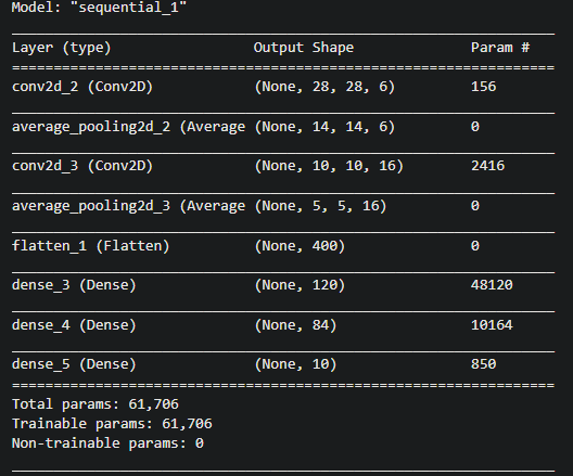
def LeNet5(input_shape=(28,28,1)):
model = keras.Sequential([
keras.Input(shape=input_shape),
layers.Conv2D(filters=6, kernel_size=(5,5), padding='same', activation='sigmoid'),
layers.AveragePooling2D(pool_size=(2,2), strides=(2,2), padding='valid'),
layers.Conv2D(filters=16, kernel_size=(5,5), padding='valid', activation='sigmoid'),
layers.AveragePooling2D(pool_size=(2,2), strides=(2,2), padding='valid'),
layers.Flatten(),#二维拉平为一维
layers.Dense(units=120, activation='sigmoid'),
layers.Dense(units=84, activation='sigmoid'),
layers.Dense(units=10, activation='softmax')
])
model.compile(
optimizer='adam',
loss='categorical_crossentropy',
metrics=['categorical_accuracy']
)
return model
model= LeNet5()
model.summary()
加载数据集、数据集标准化、划分数据集、one-hot编码
import tensorflow as tf
import numpy as np
from sklearn.model_selection import train_test_split

# 1. Load the MNIST dataset
mnist = tf.keras.datasets.mnist
(X_train_full, y_train_full), (X_test_original, y_test_original) = mnist.load_data()

# 2. Normalize image data to a [0, 1] range
X_train_full = X_train_full.astype('float32') / 255.0
X_test_original = X_test_original.astype('float32') / 255.0

# 3. Print initial data dimensions
print('Full Training data dimensions:', X_train_full.shape)
print('Original Test data dimensions:', X_test_original.shape)

# 4. Split the full training dataset into new training and validation sets
# This creates a 80/20 split from the original training data
X_train, X_val, y_train, y_val = train_test_split(
    X_train_full, y_train_full, test_size=0.2, random_state=0
)

# 5. Print new training, validation, and original test dimensions
print('\nNew Training data dimensions:', X_train.shape)
print('Validation data dimensions:', X_val.shape)
print('Original Test data dimensions:', X_test_original.shape)

# 6. One-hot encode the labels for the training and validation sets
# MNIST has 10 classes (digits 0-9)
num_classes = 10
y_train_one_hot = tf.keras.utils.to_categorical(y_train, num_classes=num_classes)
y_val_one_hot = tf.keras.utils.to_categorical(y_val, num_classes=num_classes)
# Note: y_test_original is not one-hot encoded here as it's not used in subsequent training/validation steps in the notebook

# 7. Print shapes and examples of one-hot encoded labels
print('\nOriginal y_train shape:', y_train.shape)
print('One-hot encoded y_train shape:', y_train_one_hot.shape)
print('\nFirst 5 original labels from y_train:', y_train[:5])
print('First 5 one-hot encoded labels from y_train:\n', y_train_one_hot[:5])

# 8. Reshape image data to include the channel dimension (for CNN input)
# Images are 28x28 grayscale, so the shape becomes (num_samples, 28, 28, 1)
print('\nCurrent X_train shape before reshaping:', X_train[:1].shape)
X_train = X_train.reshape(-1, 28, 28, 1)
X_val = X_val.reshape(-1, 28, 28, 1)
# The original X_test_original is not used for validation in the subsequent cells, X_val is used instead.
# If X_test_original were to be used for final evaluation, it would also need reshaping:
# X_test_original = X_test_original.reshape(-1, 28, 28, 1)

print('Reshaped X_train dimensions:', X_train.shape)
print('Reshaped X_val dimensions:', X_val.shape)
训练
# 创建模型
model = LeNet5()
# Early stopping 防止过拟合
early_stopping = keras.callbacks.EarlyStopping(
    patience = 10,#defines the number of epochs the training will continue after the monitored metric has stopped improving.
    min_delta = 0.0001,#the minimum change in the monitored metric that qualifies as an "improvement."
    restore_best_weights=True,#停止时权重为迄今为止最好的
)
# Train model
#history包含训练时的指标,如损失,精度等
history = model.fit(
    X_train,y_train_one_hot,
    validation_data=(X_val,y_val_one_hot),
    batch_size=32,
    epochs=200,
    callbacks=[early_stopping],
    verbose=True
)
评估
#预测
preds = model.predict(X_val) #predict() method outputs an array of probabilities for each class (0-9) for every image
# print(preds[:20])
# In NumPy, axis=0 refers to the rows (or the first dimension).
# axis=1 refers to the columns (or the second dimension).
conf= np.max(preds,axis=1) #所以这个返回的就是每列概率最高的值
pred_classes = np.argmax(preds, axis=1)#这个返回的是每列概率最高的值的索引 对于one-hot来说就是标签

# print(pred_classes)
#Plot some model predictions
plt.figure(figsize=(15,4))
plt.suptitle('Model predictions', fontsize=20, y=1.05)

# Subplot
for i in range(20):
    img = X_val[i].reshape((28,28))/255;
    ax=plt.subplot(2, 10, i+1)
    ax.grid(False)
    ax.get_xaxis().set_visible(False)
    ax.get_yaxis().set_visible(False)
    ax.set_title(f'Pred:{pred_classes[i]} \n Conf:{np.round(100*conf[i],1)}', fontdict = {'fontsize':14})
    plt.imshow(img, cmap='gray')

plt.show()
测试结果

获取损失和精确度
# 这里选取了训练集和测试集的损失,准确率
history_df = pd.DataFrame(history.history)
history_df.loc[:, ['loss', 'val_loss']].plot(title="Cross-entropy")
history_df.loc[:, ['categorical_accuracy', 'val_categorical_accuracy']].plot(title="Accuracy")

print('Final accuracy on validation set:', history_df.loc[len(history_df)-1,'val_categorical_accuracy'])
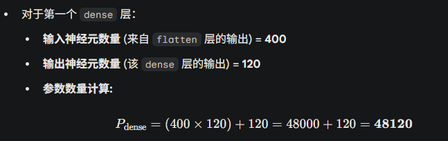
Dense层处理后参数剧增
参数计算公式:
AlexNet
为了适配CIFAR-10的10分类任务,对输入大小、卷积核大小和数量、步幅、优化器、填充、每层神经元个数,进行了更改,每个卷积后加入一个BatchNormalization,卷积中加入regularizers。
这种修改称为结构定制。
import tensorflow as tf
from tensorflow import keras
from tensorflow.keras import layers, models, regularizers,optimizers

# 定义为 CIFAR-10 优化的 AlexNet 模型
def build_alexnet_cifar10_optimized(input_shape=(32, 32, 3), num_classes=10):

    # 使用 Sequential 模型容器
    model = models.Sequential([
        tf.keras.Input(shape=input_shape),

        # ------------------ Conv Layer 1 ------------------
        # 调整为 5x5, Stride=1, 避免 32x32 图像信息流失过快
        layers.Conv2D(
            filters=64,
            kernel_size=(5, 5),
            strides=(1, 1),
            padding='same',
            activation='relu',
            kernel_regularizer=regularizers.l2(0.0005)
        ),
        layers.BatchNormalization(),
        layers.MaxPool2D(pool_size=(2, 2), strides=(2, 2)), # 32 -> 16

        # ------------------ Conv Layer 2 ------------------
        # 注意:第二个卷积层在 Keras 中默认 strides=(1,1)
        layers.Conv2D(
            filters=192,
            kernel_size=(5, 5),
            padding='same',
            activation='relu',
            kernel_regularizer=regularizers.l2(0.0005)
        ),
        layers.BatchNormalization(),
        layers.MaxPool2D(pool_size=(2, 2), strides=(2, 2)), # 16 -> 8

        # ------------------ Conv Layer 3 ------------------
        layers.Conv2D(
            filters=384,
            kernel_size=(3, 3),
            padding='same',
            activation='relu',
            kernel_regularizer=regularizers.l2(0.0005)
        ),
        layers.BatchNormalization(),

        # ------------------ Conv Layer 4 ------------------
        layers.Conv2D(
            filters=256,
            kernel_size=(3, 3),
            padding='same',
            activation='relu',
            kernel_regularizer=regularizers.l2(0.0005)
        ),
        layers.BatchNormalization(),

        # ------------------ Conv Layer 5 ------------------
        layers.Conv2D(
            filters=256,
            kernel_size=(3, 3),
            padding='same',
            activation='relu',
            kernel_regularizer=regularizers.l2(0.0005)
        ),
        layers.BatchNormalization(),
        layers.MaxPool2D(pool_size=(2, 2), strides=(2, 2)), # 8 -> 4

        # ------------------ 全连接层 (Dense Layers) ------------------
        layers.Flatten(),

        # Dense 6 (Units 调整以适应小数据集)
        layers.Dense(1024, activation='relu'),
        layers.Dropout(0.5), # 标准 AlexNet/深度网络实践

        # Dense 7
        layers.Dense(1024, activation='relu'),
        layers.Dropout(0.5),

        # Dense 8 (输出层)
        layers.Dense(num_classes, activation='softmax')
    ])

    return model

# 示例:创建模型并打印摘要
model = build_alexnet_cifar10_optimized()
model.summary()
处理测试集
import numpy as np
import tensorflow as tf
from tensorflow.keras.datasets import cifar10
(x_train,y_train),(x_test,y_test) = cifar10.load_data()
# 2. 数据标准化/归一化到 [0, 1]
x_train = x_train.astype('float32') / 255.0
x_test = x_test.astype('float32') / 255.0

# 3. 确定输入形状和类别数
INPUT_SHAPE = x_train.shape[1:]  # (32, 32, 3)
NUM_CLASSES = 10

print(f"训练集形状: {x_train.shape}")
print(f"测试集形状: {x_test.shape}")
训练
model = build_alexnet_cifar10_optimized(INPUT_SHAPE,NUM_CLASSES)

model.compile(
    optimizer='adam',
    loss='sparse_categorical_crossentropy',
    metrics=['accuracy']
)

early_stopping = keras.callbacks.EarlyStopping(
    patience = 10,#defines the number of epochs the training will continue after the monitored metric has stopped improving.
    min_delta = 0.0001,#the minimum change in the monitored metric that qualifies as an "improvement."
    restore_best_weights=True,#停止时权重为迄今为止最好的
)

history = model.fit(
    x_train,
    y_train,
    epochs=200,
    batch_size=32,
    validation_data=(x_test, y_test),
    callbacks=[early_stopping]
)
绘制相关数据曲线
import pandas as pd
import matplotlib.pyplot as plt

# 假设 history 是 model.fit() 返回的对象

history_df = pd.DataFrame(history.history)

plt.figure(figsize=(12, 5))

# 1. 绘制损失曲线
plt.subplot(1, 2, 1)
history_df.loc[:, ['loss', 'val_loss']].plot(ax=plt.gca())
plt.title("Cross-entropy Loss")
plt.xlabel("Epoch")
plt.ylabel("Loss")

# 2. 绘制准确率曲线 (已将 categorical_accuracy 修正为 accuracy)
plt.subplot(1, 2, 2)
history_df.loc[:, ['accuracy', 'val_accuracy']].plot(ax=plt.gca())
plt.title("Accuracy")
plt.xlabel("Epoch")
plt.ylabel("Accuracy")

plt.tight_layout()
plt.show()

# 打印最终验证集准确率 (已将 val_categorical_accuracy 修正为 val_accuracy)
final_val_accuracy = history_df.loc[len(history_df) - 1, 'val_accuracy']
print('Final accuracy on validation set:', final_val_accuracy)
展示测试
import numpy as np
import matplotlib.pyplot as plt

# -------------------------- 预测步骤 --------------------------

# 使用测试集(x_test)进行预测
# 注意:我们假设 x_test 已经被标准化到 [0, 1]
preds = model.predict(x_test)

# 获取最高概率值 (置信度)
# np.max(preds, axis=1) 返回每一行(即每个样本)中概率最高的值
conf = np.max(preds, axis=1)

# 获取预测类别索引
# np.argmax(preds, axis=1) 返回每一行中概率最高的值的索引,即预测的类别标签 (0-9)
pred_classes = np.argmax(preds, axis=1)

# -------------------------- 可视化步骤 --------------------------

# CIFAR-10 类别名称 (可选,用于更清晰的标签)
cifar10_labels = ['airplane', 'automobile', 'bird', 'cat', 'deer', 'dog', 'frog', 'horse', 'ship', 'truck']

# 绘制前 20 个样本的预测结果
NUM_SAMPLES_TO_PLOT = 20
plt.figure(figsize=(15, 4))
plt.suptitle('Model predictions on Test Data', fontsize=16, y=1.05)

# Subplot
for i in range(NUM_SAMPLES_TO_PLOT):
    # 使用测试集数据 x_test
    img_data = x_test[i]

    ax = plt.subplot(2, 10, i + 1)

    # 隐藏坐标轴
    ax.grid(False)
    ax.get_xaxis().set_visible(False)
    ax.get_yaxis().set_visible(False)

    # 设置标题:显示预测类别和置信度
    predicted_label_name = cifar10_labels[pred_classes[i]]

    # 检查预测是否正确 (可选:显示颜色)
    is_correct = (pred_classes[i] == y_test[i][0])
    color = 'green' if is_correct else 'red'

    ax.set_title(
        f'{predicted_label_name} \n Conf:{np.round(100*conf[i], 1)}%',
        fontdict={'fontsize': 10},
        color=color
    )

    # 显示图像。CIFAR-10 图像已经是 32x32x3,无需 reshape
    # 也不用再次除以 255,因为它已经被标准化
    plt.imshow(img_data)

plt.tight_layout(rect=[0, 0, 1, 0.96]) # 调整布局以适应 suptitle
plt.show()

# -------------------------- 附加信息 --------------------------
print(f"\n绿色标题表示预测正确,红色标题表示预测错误。")
感觉PyTorch的封装程度没有TensorFlow高。